Introduction
One approach for exploring and understanding user engagement is text mining. Text mining is the practice of using automated tools to examine large amounts of free-form text, summarize the contents, uncover interesting patterns, and generate new insights from the data.
The most active areas of research in text mining for health have been the analysis of electronic medical records (Koleck et al. 2019, @kreimeyer:2017) and social media messages (Sinnenberg et al. 2017). There have been few published analyses of two-way communication transcripts. Ye et al. (2010) published a systematic review of studies, which examined e-mail communication between patients and providers. Blanc et al. (2016) conducted a content analysis of messages that users in Nigeria sent to a sexual and reproductive health question and answer service called MyQuestion. Despite a large and growing body of evidence around the efficacy of text message-based interventions, there has been scant attention to the study of user engagement through text mining.
In a new paper published in Gates Open Research, we conducted a text mining analysis of the inbound and outbound messages to askNivi. The objective of this analysis was to characterize the ways that Kenyan men and women communicated with about their health inquiries to inform future content development, tailoring, and automation. I thought it would be fun to walk through our text mining analysis. We relied heavily on Text Mining with R by Julia Silge and David Robinson.
Text Mining Example
Here is an outline of the process:
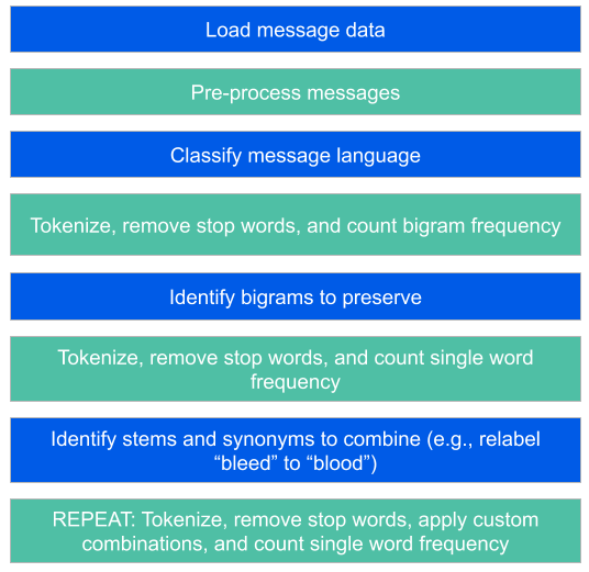
Figure 1: Text mining process.
You’ll need to download and install R and the following packages:
You’ll also need to get the example data from our data and code repository. Once you’re ready, load the dataset of English stop words, a list of custom stop words we curated, and a sample of message data.
# load stop_words from tidytext package
# -----------------------------------------------------------------------------
  data(stop_words) # load stop_words
# remove some words
  stop_words <- stop_words %>%
    filter(word!="side") # for side effects

# load custom stop words
# -----------------------------------------------------------------------------
  stop <- read.csv("input/example/stop.csv", stringsAsFactors = FALSE)

# load custom modifications
# -----------------------------------------------------------------------------
  modEng <- read.csv("input/example/modifications-en.csv",
                     stringsAsFactors = FALSE)
  modEng <- modEng %>%
    filter(rename!="")

# load sample anonymized message data
# -----------------------------------------------------------------------------
  df <- read.csv("input/example/example.csv", stringsAsFactors = FALSE)
Message data can be quite messy, so we conduct a bit of pre-processing to replace periods with spaces to separate words (e.g., “end.beginning” to “end beginning”) and convert all text to lowercase.
To detect the language of each message, we used the cld2 package [v1.2] to access Google’s Compact Language Detector 2, a Naïve Bayesian classifier that probabilistically detects 83 languages, including English and Swahili.
  df$msgLang <- cld2::detect_language(df$message_)
  df$msgLang <- ifelse(df$msgLang=="en" |            # set other langs to NA
                       df$msgLang=="sw",
                       df$msgLang, NA)
Now to the fun parts. The next step is to examine the frequency of consecutive words, bigrams. The key function is unnest_tokens() that breaks messages into pairs of words. separate() separates pairs into two columns so it’s possible to remove stop words from each column before re-uniting and counting.
  out1 <- df %>%
  # limit to incoming messages in english
    filter(msgLang=="en") %>%
  # tokenize
    unnest_tokens(word, message_, token = "ngrams", n = 2) %>%
    separate(word, c("word1", "word2"), sep = " ") %>%
  # remove stop words
    anti_join(filter(stop_words), by = c(word1 = "word")) %>%
    anti_join(filter(stop_words), by = c(word2 = "word")) %>%
    filter(!(word1 %in% stop$niviStop)) %>%
    filter(!(word2 %in% stop$niviStop)) %>%
    unite(word, word1, word2, sep = " ") %>%
  # custom spelling corrections, if necessary
    mutate(word = ifelse(word=="prostrate cancer", "prostate cancer", word)) %>%
    mutate(word = ifelse(word=="family planing", "family planning", word)) %>%
    mutate(word = ifelse(word=="planning method", "planning methods", word)) %>%
  # count
    count(word, sort = TRUE) %>%
    dplyr::select(word, n) %>%
    filter(word!="NA NA")
Here’s the result from our example data:
              word n
1    breast cancer 4
2  family planning 4
3  prostate cancer 3
4     giving birth 2
5    sexual health 2
6     side effects 2
7            3 sum 1
8   abnormal child 1
9      abov sexual 1
10       ady ngozi 1
When counting individual words, we wanted to preserve some bigrams. For instance, when the word “family” immediately preceded the word “planning”, we wanted to tally “family” as part of the bigram “family planning”. However, if “family” occurred on its own, e.g., “I do not want to start a family”, then we wanted to tally family as an individual term.
Our approach is a bit hacky, but we take all observed spellings of the bigrams and concatenate without a space, “familyplanning”. This will count instances of “familyplanning” separate from instances of “family” and “planning” that do not appear together.
  df <- df %>%
    mutate(message_ = gsub("breast cancer|breast caancer",
                           "breastcancer",
                           message_)) %>%
    mutate(message_ = gsub("family planning",
                           "familyplanning",
                           message_,
                           fixed=TRUE)) %>%
    mutate(message_ = gsub("prostate cancer",
                           "prostatecancer",
                           message_,
                           fixed=TRUE)) %>%
    mutate(message_ = gsub("sexual health",
                           "sexualhealth",
                           message_,
                           fixed=TRUE))

  bigramKeep <- c("breastcancer", "familyplanning", "prostatecancer",
                  "sexualhealth"
  )
The next example shows how to tokenize messages and count the frequency of individual words. This approach can be modified with group_by() functions (#commented out below) to count frequency of words by group.
Text Mining with R gives a simpler, cleaner example of how to conduct this analysis. Our approach will likely work for new examples, but the specifics may be somewhat unique to the challenges we observed in our message data.
We ran this process an initial time and used the results to make a custom list of modifications to incorporate into final processing.
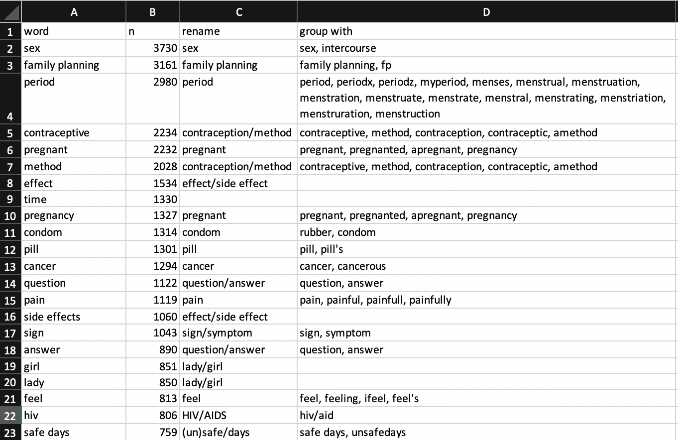
Figure 2: Custom modifications.
For instance, we wanted to collapse all instances of the words “sex” and “intercourse” into the word “sex”. This is a step beyond lemmatization (shown below) that collapses words into lemma, e.g., “prenancy” to “pregnant”.
  out2 <- df %>%
  # limit to incoming messages in english
    filter(msgLang=="en") %>%

  # tokenize
  # ---------------------------------------------------------------------------
  # to tokenize by group, add group_by
  # group_by(genAge) %>%
    unnest_tokens(word, message_) %>%

  # get initial count
    count(word, sort = TRUE) %>%
  # remove numbers and punctuation from strings
    mutate(word = gsub('[[:digit:]]+', '', word)) %>%
    mutate(word = gsub('_', '', word)) %>%
    mutate(word = gsub(',', '', word)) %>%
  # remove blank or 1 character after number removal
    filter(nchar(word)>1) %>%

  # spelling, lemmatization
  # ---------------------------------------------------------------------------
  # suggest spelling replacements
    mutate(suggest = unlist(lapply(hunspell_suggest(word),
                                   function(x) x[1]))) %>%
  # keep spelling suggestion for words where n < ??
  # mutate(word = ifelse(n<??, suggest, word)) %>%  # turned off to ignore
  # correct a few problems hunspell introduces in these replacements
    mutate(word = tolower(word)) %>%
    mutate(word = gsub(" ", "", word)) %>%
  # lemma
    mutate(lemma = lemmatize_words(word)) %>%
  # keep lemma unless word is in bigramKeep
    mutate(word = ifelse((word %in% bigramKeep), suggest, lemma)) %>%
  # another round of corrections
    mutate(word = gsub('[[:digit:]]+', '', word)) %>%
    filter(!is.na(word)) %>%
    filter(word!="") %>%

  # recount
  # ---------------------------------------------------------------------------
    dplyr::select(-lemma) %>%  #-suggest, -stem,
    group_by(word) %>%   # if tokenized by group: group_by(genAge, word) %>%
    summarise(n = sum(n)) %>%
    arrange(desc(n)) %>%

  # custom modifications (revert lemma, combine synonmyms)
  # ---------------------------------------------------------------------------
    left_join( dplyr::select(modEng, word, rename), by="word") %>%
    mutate(word = ifelse(!is.na(rename), rename, word)) %>%
    dplyr::select(-rename) %>%

  # recount
  # ---------------------------------------------------------------------------
    group_by(word) %>%  # if tokenized by group: group_by(genAge, word) %>%
    summarise(n = sum(n)) %>%
    arrange(desc(n)) %>%
  # remove stop words again
    anti_join(stop_words) %>%
    filter(!(word %in% stop$niviStop))
Here’s the result from our example data:
# A tibble: 10 x 2
   word                     n
   <chr>                <int>
 1 contraception/method    12
 2 sex                      8
 3 period                   7
 4 age                      6
 5 safe                     6
 6 sexual                   6
 7 sign/symptom             6
 8 blood/bleed              4
 9 cancer                   4
10 effect/side effect       4
These results can be piped to the visualization code as shown in the manuscript.Rmd file in the data and code repository. There you’ll also find the data and code you need to reproduce the full paper.
Full paper
Green EP, Whitcomb A, Kahumbura C et al. “What is the best method of family planning for me?”: a text mining analysis of messages between users and agents of a digital health service in Kenya [version 1; peer review: 2 approved]. Gates Open Res 2019, 3:1475
DOI: 10.12688/gatesopenres.12999.1
PMID: 31410395
PMCID: PMC6688461
Data and Code
You can find the data and code for this paper here.
Blanc, Ann K., Kimberly Glazer, Uju Ofomata-Aderemi, and Fadekemi Akinfaderin-Agarau. 2016. “Myths and Misinformation: An Analysis of Text Messages Sent to a Sexual and Reproductive Health Q&A Service in Nigeria.” Studies in Family Planning 47 (1): 39–53.
Koleck, Theresa A., Caitlin Dreisbach, Philip E. Bourne, and Suzanne Bakken. 2019. “Natural Language Processing of Symptoms Documented in Free-Text Narratives of Electronic Health Records: A Systematic Review.” Journal of the American Medical Informatics Association 26 (4): 364–79. https://doi.org/10.1093/jamia/ocy173.
Kreimeyer, Kory, Matthew Foster, Abhishek Pandey, Nina Arya, Gwendolyn Halford, Sandra F. Jones, Richard Forshee, Mark Walderhaug, and Taxiarchis Botsis. 2017. “Natural Language Processing Systems for Capturing and Standardizing Unstructured Clinical Information: A Systematic Review.” Journal of Biomedical Informatics 73: 14–29.
Nivi. 2018. “AskNivi.” http://www.webcitation.org/77zqfMqGn.
Sinnenberg, Lauren, Alison M. Buttenheim, Kevin Padrez, Christina Mancheno, Lyle Ungar, and Raina M. Merchant. 2017. “Twitter as a Tool for Health Research: A Systematic Review.” American Journal of Public Health 107 (1): e1–e8.
Ye, Jiali, George Rust, Yvonne Fry-Johnson, and Harry Strothers. 2010. “E-Mail in Patient–Provider Communication: A Systematic Review.” Patient Education and Counseling 80 (2): 266–73.